
![Coursera: Neural Networks and Deep Learning (Week 3) [Assignment Solution] - deeplearning.ai | APDaga | DumpBox](https://blogger.googleusercontent.com/img/b/R29vZ2xl/AVvXsEi5t2_iG4WhBKsL-oN2M7XlliwvnsQxnhbaXyU5OOQfBc81B-0XlHSXi-ExpObgEDFrqkJKkROJZ9k4DDPVjcpKRQmc9F0WHcdcSJO4vXDBSEFwmq3drk39nNSC0DuAQsgjtpVyMheh2U4/s320/NN+week3+thumbnail-min.jpg "Coursera: Neural Networks and Deep Learning (Week 3) [Assignment Solution] - deeplearning.ai | APDaga | DumpBox")
▸ Planar data classification with one hidden layer.
I have recently completed the Neural Networks and Deep Learning course from Coursera by deeplearning.ai
While doing the course we have to go through various quiz and assignments in Python.
Here, I am sharing my solutions for the weekly assignments throughout the course.
> It is recommended that you should solve the assignments by yourself honestly then only it makes sense to complete the course.
> But, In case you stuck in between, feel free to refer to the solutions provided by me.
![Coursera: Neural Networks and Deep Learning (Week 3) [Assignment Solution] - deeplearning.ai | APDaga | DumpBox](https://blogger.googleusercontent.com/img/b/R29vZ2xl/AVvXsEi5t2_iG4WhBKsL-oN2M7XlliwvnsQxnhbaXyU5OOQfBc81B-0XlHSXi-ExpObgEDFrqkJKkROJZ9k4DDPVjcpKRQmc9F0WHcdcSJO4vXDBSEFwmq3drk39nNSC0DuAQsgjtpVyMheh2U4/s1600/NN+week3+thumbnail-min.jpg "Coursera: Neural Networks and Deep Learning (Week 3) [Assignment Solution] - deeplearning.ai | APDaga | DumpBox") |
I have recently completed the Neural Networks and Deep Learning course from Coursera by deeplearning.ai
NOTE:
Don't just copy paste the code for the sake of completion.
Even if you copy the code, make sure you understand the code first.
Click Here: Coursera: Neural Networks & Deep Learning (Week 2)
Click Here: Coursera: Neural Networks & Deep Learning (Week 4A)
Scroll down for Coursera: Neural Networks & Deep Learning (Week 3) Assignments.
Recommended Machine Learning Courses:- Coursera: Machine Learning
- Coursera: Deep Learning Specialization
- Coursera: Machine Learning with Python
- Coursera: Advanced Machine Learning Specialization
- Udemy: Machine Learning
- LinkedIn: Machine Learning
- Eduonix: Machine Learning
- edX: Machine Learning
- Fast.ai: Introduction to Machine Learning for Coders
Even if you copy the code, make sure you understand the code first.
Click Here: Coursera: Neural Networks & Deep Learning (Week 2)
Click Here: Coursera: Neural Networks & Deep Learning (Week 4A)
Scroll down for Coursera: Neural Networks & Deep Learning (Week 3) Assignments.Recommended Machine Learning Courses:
- Coursera: Machine Learning
- Coursera: Deep Learning Specialization
- Coursera: Machine Learning with Python
- Coursera: Advanced Machine Learning Specialization
- Udemy: Machine Learning
- LinkedIn: Machine Learning
- Eduonix: Machine Learning
- edX: Machine Learning
- Fast.ai: Introduction to Machine Learning for Coders
Planar data classification with one hidden layer
Welcome to your week 3 programming assignment. It's time to build your first neural network, which will have a hidden layer. You will see a big difference between this model and the one you implemented using logistic regression.
You will learn how to:
- Implement a 2-class classification neural network with a single hidden layer
- Use units with a non-linear activation function, such as tanh
- Compute the cross entropy loss
- Implement forward and backward propagation
1 - Packages
Let's first import all the packages that you will need during this assignment.
- numpy is the fundamental package for scientific computing with Python.
- sklearn provides simple and efficient tools for data mining and data analysis.
- matplotlib is a library for plotting graphs in Python.
- testCases provides some test examples to assess the correctness of your functions
- planar_utils provide various useful functions used in this assignment
In [1]:
2 - Dataset
First, let's get the dataset you will work on. The following code will load a "flower" 2-class dataset into variables
X and Y.
In [2]:
Visualize the dataset using matplotlib. The data looks like a "flower" with some red (label y=0) and some blue (y=1) points. Your goal is to build a model to fit this data.
In [3]:
You have:
- a numpy-array (matrix) X that contains your features (x1, x2)
- a numpy-array (vector) Y that contains your labels (red:0, blue:1).
Lets first get a better sense of what our data is like.
Exercise: How many training examples do you have? In addition, what is the
shape of the variables X and Y?
Hint: How do you get the shape of a numpy array? (help)
In [4]:
Expected Output:
| shape of X | (2, 400) |
| shape of Y | (1, 400) |
| m | 400 |
3 - Simple Logistic Regression
Before building a full neural network, lets first see how logistic regression performs on this problem. You can use sklearn's built-in functions to do that. Run the code below to train a logistic regression classifier on the dataset.
In [5]:
You can now plot the decision boundary of these models. Run the code below.
In [6]:
Expected Output:
| Accuracy | 47% |
Interpretation: The dataset is not linearly separable, so logistic regression doesn't perform well. Hopefully a neural network will do better. Let's try this now!
Check-out our free tutorials on IOT (Internet of Things):
4 - Neural Network model
Logistic regression did not work well on the "flower dataset". You are going to train a Neural Network with a single hidden layer.
Here is our model:

Mathematically:
For one example :

Given the predictions on all the examples, you can also compute the cost as follows:
J=−1m∑i=0m(y(i)log(a[2](i))+(1−y(i))log(1−a[2](i))) (6)
4.1 - Defining the neural network structur

Given the predictions on all the examples, you can also compute the cost as follows:
J=−1m∑i=0m(y(i)log(a[2](i))+(1−y(i))log(1−a[2](i))) (6)
Reminder: The general methodology to build a Neural Network is to:
1. Define the neural network structure ( # of input units,  # of hidden units, etc).
2. Initialize the model's parameters
3. Loop:
    - Implement forward propagation
    - Compute loss
    - Implement backward propagation to get the gradients
    - Update parameters (gradient descent)
You often build helper functions to compute steps 1-3 and then merge them into one function we call
nn_model(). Once you've built nn_model() and learnt the right parameters, you can make predictions on new data.4.1 - Defining the neural network structure
Exercise: Define three variables:
- n_x: the size of the input layer
- n_h: the size of the hidden layer (set this to 4)
- n_y: the size of the output layer
Hint: Use shapes of X and Y to find n_x and n_y. Also, hard code the hidden layer size to be 4.
In [7]:
In [8]:
Out [8]:
Expected Output (these are not the sizes you will use for your network, they are just used to assess the function you've just coded).
Expected Output (these are not the sizes you will use for your network, they are just used to assess the function you've just coded).
| n_x | 5 |
| n_h | 4 |
| n_y | 2 |
4.2 - Initialize the model's parameters
Exercise: Implement the function
initialize_parameters().
Instructions:
- Make sure your parameters' sizes are right. Refer to the neural network figure above if needed.
- You will initialize the weights matrices with random values.
- Use:
np.random.randn(a,b) * 0.01to randomly initialize a matrix of shape (a,b).
- Use:
- You will initialize the bias vectors as zeros.
- Use:
np.zeros((a,b))to initialize a matrix of shape (a,b) with zeros.
In [9]:
In [10]:
Out [10]:
Expected Output:
W1
|
[[-0.00416758 -0.00056267] [-0.02136196 0.01640271] [-0.01793436 -0.00841747]
[ 0.00502881 -0.01245288]]
|
b1
|
[[ 0.] [ 0.] [ 0.] [ 0.]]
|
W2
|
[[-0.01057952 -0.00909008 0.00551454 0.02292208]]
|
b2
|
[[ 0.]]
|
4.3 - The Loop
Question: Implement
forward_propagation().
Instructions:
- Look above at the mathematical representation of your classifier.
- You can use the function
sigmoid(). It is built-in (imported) in the notebook. - You can use the function
np.tanh(). It is part of the numpy library. - The steps you have to implement are:
- Retrieve each parameter from the dictionary "parameters" (which is the output of
initialize_parameters()) by usingparameters[".."]. - Implement Forward Propagation. Compute and (the vector of all your predictions on all the examples in the training set).
- Retrieve each parameter from the dictionary "parameters" (which is the output of
- Values needed in the backpropagation are stored in "
cache". Thecachewill be given as an input to the backpropagation function.
In [11]:
# GRADED FUNCTION: forward_propagation

def forward_propagation(X, parameters):
    """
    Argument:
    X -- input data of size (n_x, m)
    parameters -- python dictionary containing your parameters (output of initialization function)

    Returns:
    A2 -- The sigmoid output of the second activation
    cache -- a dictionary containing "Z1", "A1", "Z2" and "A2"
    """
    # Retrieve each parameter from the dictionary "parameters"
    ### START CODE HERE ### (≈ 4 lines of code)
    W1 = parameters["W1"]  # (4,2)
    b1 = parameters["b1"]  # (4,1)
    W2 = parameters["W2"]  # (1,4)
    b2 = parameters["b2"]  # (1,1)
    ### END CODE HERE ###

    # Implement Forward Propagation to calculate A2 (probabilities)
    ### START CODE HERE ### (≈ 4 lines of code)
    Z1 = np.dot(W1,X) + b1
    A1 = np.tanh(Z1)
    Z2 = np.dot(W2,A1) + b2
    A2 = sigmoid(Z2)
    ### END CODE HERE ###

    #print("W1_shape = "+ str(W1.shape))
    #print("b1_shape = "+ str(b1.shape))
    #print("W2_shape = "+ str(W2.shape))
    #print("b2_shape = "+ str(b2.shape))
    #print("X_shape  = "+ str(X.shape))
    #print("Z1_shape = "+ str(Z1.shape))
    #print("A1_shape = "+ str(A1.shape))
    #print("Z2_shape = "+ str(Z2.shape))
    #print("A2_shape = "+ str(A2.shape))


    assert(A2.shape == (1, X.shape[1]))

    cache = {"Z1": Z1,
             "A1": A1,
             "Z2": Z2,
             "A2": A2}

    return A2, cache
In [12]:
Out [12]:
Expected Output:
| 0.262818640198 0.091999045227 -1.30766601287 0.212877681719 |
Now that you have computed (in the Python variable "
J=−1m∑i=0m(y(i)log(a[2](i))+(1−y(i))log(1−a[2](i))) (13)
A2"), which contains for every example, you can compute the cost function as followsJ=−1m∑i=0m(y(i)log(a[2](i))+(1−y(i))log(1−a[2](i))) (13)
Exercise: Implement
compute_cost() to compute the value of the cost .
Instructions:
- There are many ways to implement the cross-entropy loss. To help you, we give you how we would have implemented :
logprobs = np.multiply(np.log(A2),Y)
cost = - np.sum(logprobs)                # no need to use a for loop!
(you can use either
np.multiply() and then np.sum() or directly np.dot()).
In [13]:
In [14]:
Out [14]:
Expected Output:
| cost | 0.693058761... |
Using the cache computed during forward propagation, you can now implement backward propagation.
Question: Implement the function
backward_propagation().
Instructions: Backpropagation is usually the hardest (most mathematical) part in deep learning. To help you, here again is the slide from the lecture on backpropagation. You'll want to use the six equations on the right of this slide, since you are building a vectorized implementation.

Tips:
- To compute dZ1 you'll need to compute . Since is the tanh activation function, if then . So you can compute using
(1 - np.power(A1, 2)).
In [15]:
# GRADED FUNCTION: backward_propagation

def backward_propagation(parameters, cache, X, Y):
    """
    Implement the backward propagation using the instructions above.

    Arguments:
    parameters -- python dictionary containing our parameters
    cache -- a dictionary containing "Z1", "A1", "Z2" and "A2".
    X -- input data of shape (2, number of examples)
    Y -- "true" labels vector of shape (1, number of examples)

    Returns:
    grads -- python dictionary containing your gradients with respect to different parameters
    """
    m = X.shape[1]

    # First, retrieve W1 and W2 from the dictionary "parameters".
    ### START CODE HERE ### (≈ 2 lines of code)
    W1 = parameters["W1"]
    W2 = parameters["W2"]
    ### END CODE HERE ###

    # Retrieve also A1 and A2 from dictionary "cache".
    ### START CODE HERE ### (≈ 2 lines of code)
    A1 = cache["A1"]
    A2 = cache["A2"]
    ### END CODE HERE ###

    # Backward propagation: calculate dW1, db1, dW2, db2.

    # Here, n_x = 2
    #       n_h = 4
    #       n_y = 1

    # X = (2,3)  Y = (1,3)  A2 = (1,3)   A1 = (4,3)

    #print("X_shape = "+str(X.shape))
    #print("Y_shape = "+str(Y.shape))
    #print("A1_shape = "+str(A1.shape))
    #print("A2_shape = "+str(A2.shape))

    ### START CODE HERE ### (≈ 6 lines of code, corresponding to 6 equations on slide above)
    dZ2 = A2 - Y                                        # (1,3)
    dW2 = (1/m) * np.dot(dZ2,A1.T)                      # (1,4) = (1,3).(3,4)
    db2 = (1/m) * np.sum(dZ2, axis=1, keepdims=True)    # (1,1) = sum(1,3)

    dZ1 = np.dot(W2.T,dZ2) * (1 - np.power(A1,2))       # (4,3) = (4,1).(1,3)
    dW1 = (1/m) * np.dot(dZ1,X.T)                       # (4,2) = (4,3).(3,2)
    db1 = (1/m) * np.sum(dZ1, axis=1, keepdims=True)    # (4,1) = sum(4,3)
    ### END CODE HERE ###

    #print("dZ2_shape = "+str(dZ2.shape))
    #print("dW2_shape = "+str(dW2.shape))
    #print("db2_shape = "+str(db2.shape))
    #print("dZ1_shape = "+str(dZ1.shape))
    #print("dW1_shape = "+str(dW1.shape))
    #print("db1_shape = "+str(db1.shape))


    grads = {"dW1": dW1,
             "db1": db1,
             "dW2": dW2,
             "db2": db2}

    return grads
In [16]:
Out [16]:
Expected output:
Expected output:
dW1
|
[[ 0.00301023 -0.00747267] [ 0.00257968 -0.00641288] [-0.00156892 0.003893 ]
[-0.00652037 0.01618243]]
|
db1
|
[[ 0.00176201] [ 0.00150995] [-0.00091736] [-0.00381422]]
|
dW2
|
[[ 0.00078841 0.01765429 -0.00084166 -0.01022527]]
|
db2
|
[[-0.16655712]]
|
Question: Implement the update rule. Use gradient descent. You have to use (dW1, db1, dW2, db2) in order to update (W1, b1, W2, b2).
General gradient descent rule: where is the learning rate and represents a parameter.
Illustration: The gradient descent algorithm with a good learning rate (converging) and a bad learning rate (diverging). Images courtesy of Adam Harley.


In [17]:
# GRADED FUNCTION: update_parameters

def update_parameters(parameters, grads, learning_rate = 1.2):
    """
    Updates parameters using the gradient descent update rule given above

    Arguments:
    parameters -- python dictionary containing your parameters
    grads -- python dictionary containing your gradients

    Returns:
    parameters -- python dictionary containing your updated parameters
    """
    # Retrieve each parameter from the dictionary "parameters"
    ### START CODE HERE ### (≈ 4 lines of code)
    W1 = parameters["W1"]
    b1 = parameters["b1"]
    W2 = parameters["W2"]
    b2 = parameters["b2"]
    ### END CODE HERE ###

    # Retrieve each gradient from the dictionary "grads"
    ### START CODE HERE ### (≈ 4 lines of code)
    dW1 = grads["dW1"]
    db1 = grads["db1"]
    dW2 = grads["dW2"]
    db2 = grads["db2"]
    ## END CODE HERE ###

    # Update rule for each parameter
    ### START CODE HERE ### (≈ 4 lines of code)
    W1 = W1 - learning_rate * dW1
    b1 = b1 - learning_rate * db1
    W2 = W2 - learning_rate * dW2
    b2 = b2 - learning_rate * db2
    ### END CODE HERE ###

    parameters = {"W1": W1,
                  "b1": b1,
                  "W2": W2,
                  "b2": b2}

    return parameters
In [18]:
Out [18]:
Expected Output:
Expected Output:
W1
|
[[-0.00643025 0.01936718] [-0.02410458 0.03978052] [-0.01653973 -0.02096177]
[ 0.01046864 -0.05990141]]
|
b1
|
[[ -1.02420756e-06] [ 1.27373948e-05] [ 8.32996807e-07] [ -3.20136836e-06]]
|
W2
|
[[-0.01041081 -0.04463285 0.01758031 0.04747113]]
|
b2
|
[[ 0.00010457]]
|
4.4 - Integrate parts 4.1, 4.2 and 4.3 in nn_model()
Question: Build your neural network model in
nn_model().
Instructions: The neural network model has to use the previous functions in the right order.
In [19]:
# GRADED FUNCTION: nn_model

def nn_model(X, Y, n_h, num_iterations = 10000, print_cost=False):
    """
    Arguments:
    X -- dataset of shape (2, number of examples)
    Y -- labels of shape (1, number of examples)
    n_h -- size of the hidden layer
    num_iterations -- Number of iterations in gradient descent loop
    print_cost -- if True, print the cost every 1000 iterations

    Returns:
    parameters -- parameters learnt by the model. They can then be used to predict.
    """

    np.random.seed(3)
    n_x = layer_sizes(X, Y)[0]
    n_y = layer_sizes(X, Y)[2]

    # Initialize parameters, then retrieve W1, b1, W2, b2. Inputs: "n_x, n_h, n_y". Outputs = "W1, b1, W2, b2, parameters".
    ### START CODE HERE ### (≈ 5 lines of code)
    parameters = initialize_parameters(n_x, n_h, n_y)
    W1 = parameters["W1"]
    b1 = parameters["b1"]
    W2 = parameters["W2"]
    b2 = parameters["b2"]
    ### END CODE HERE ###

    # Loop (gradient descent)

    for i in range(0, num_iterations):

        ### START CODE HERE ### (≈ 4 lines of code)
        # Forward propagation. Inputs: "X, parameters". Outputs: "A2, cache".
        A2, cache = forward_propagation(X, parameters)

        # Cost function. Inputs: "A2, Y, parameters". Outputs: "cost".
        cost = compute_cost(A2, Y, parameters)

        # Backpropagation. Inputs: "parameters, cache, X, Y". Outputs: "grads".
        grads = backward_propagation(parameters, cache, X, Y)

        # Gradient descent parameter update. Inputs: "parameters, grads". Outputs: "parameters".
        parameters = update_parameters(parameters, grads)

        ### END CODE HERE ###

        # Print the cost every 1000 iterations
        if print_cost and i % 1000 == 0:
            print ("Cost after iteration %i: %f" %(i, cost))

    return parameters
In [20]:
Out [20]:
Expected Output:
Expected Output:
cost after iteration 0
|
0.692739
|
⋮
⋮
|
⋮
⋮
|
W1
|
[[-0.65848169 1.21866811] [-0.76204273 1.39377573]
[ 0.5792005 -1.10397703] [ 0.76773391 -1.41477129]]
|
b1
|
[[ 0.287592 ] [ 0.3511264 ] [-0.2431246 ] [-0.35772805]]
|
W2
|
[[-2.45566237 -3.27042274 2.00784958 3.36773273]]
|
b2
|
[[ 0.20459656]]
|
4.5 Predictions
Question: Use your model to predict by building predict(). Use forward propagation to predict results.
 As an example, if you would like to set the entries of a matrix X to 0 and 1 based on a threshold you would do:

X_new = (X > threshold)
In [21]:
In [22]:
Out [22]:
Expected Output:
| predictions mean | 0.666666666667 |
It is time to run the model and see how it performs on a planar dataset. Run the following code to test your model with a single hidden layer of hidden units.
In [23]:
Out [23]:

Expected Output:
| Cost after iteration 9000 | 0.218607 |
In [24]:
Out [24]:
Expected Output:
Expected Output:
| Accuracy | 90% |
Accuracy is really high compared to Logistic Regression. The model has learnt the leaf patterns of the flower! Neural networks are able to learn even highly non-linear decision boundaries, unlike logistic regression.
Now, let's try out several hidden layer sizes.
4.6 - Tuning hidden layer size (optional/ungraded exercise)
Run the following code. It may take 1-2 minutes. You will observe different behaviors of the model for various hidden layer sizes.
In [25]:
Out [25]:
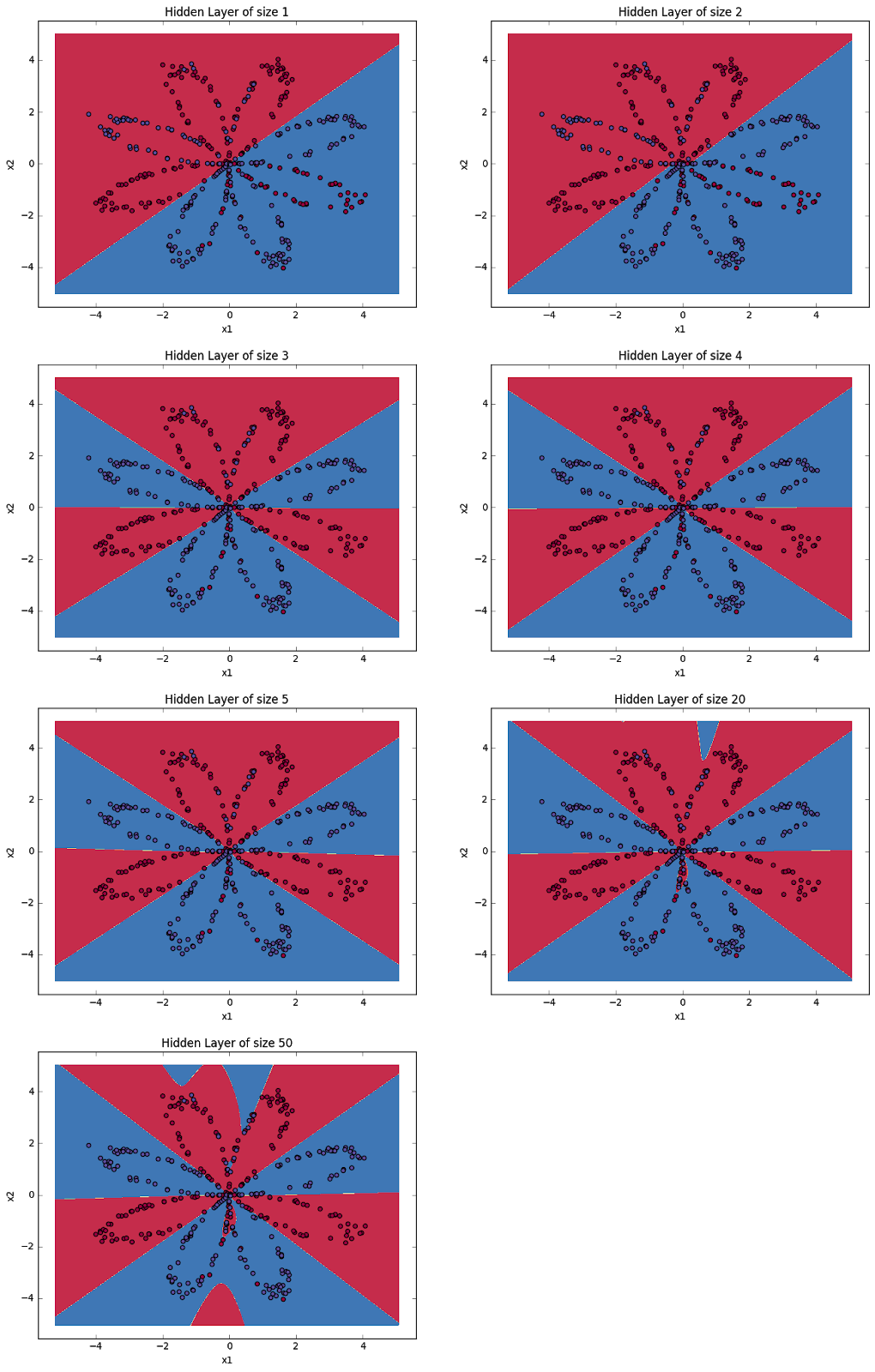
Interpretation:
- The larger models (with more hidden units) are able to fit the training set better, until eventually the largest models overfit the data.
- The best hidden layer size seems to be around n_h = 5. Indeed, a value around here seems to fits the data well without also incurring noticable overfitting.
- You will also learn later about regularization, which lets you use very large models (such as n_h = 50) without much overfitting.
Optional questions:
Note: Remember to submit the assignment but clicking the blue "Submit Assignment" button at the upper-right.
Some optional/ungraded questions that you can explore if you wish:
- What happens when you change the tanh activation for a sigmoid activation or a ReLU activation?
- Play with the learning_rate. What happens?
- What if we change the dataset? (See part 5 below!)
You've learnt to:
- Build a complete neural network with a hidden layer
- Make a good use of a non-linear unit
- Implemented forward propagation and backpropagation, and trained a neural network
- See the impact of varying the hidden layer size, including overfitting.
Nice work!
5) Performance on other datasets
If you want, you can rerun the whole notebook (minus the dataset part) for each of the following datasets.
In [26]:
Out [26]:

Congrats on finishing this Programming Assignment!
Reference:
I tried to provide optimized solutions like vectorized implementation for each assignment. If you think that more optimization can be done, then suggest the corrections / improvements in the comments.
--------------------------------------------------------------------------------
Click here to see solutions for all Machine Learning Coursera Assignments.
&
Feel free to ask doubts in the comment section. I will try my best to solve it.
If you find this helpful by any mean like, comment and share the post.
This is the simplest way to encourage me to keep doing such work.
Thanks and Regards,
-Akshay P. Daga
You can get the course's at minimal costs. Some of the courses on Coursera are free as well.
ReplyDeleteYou can also apply for free aid or audit the coursers on Coursrera itself.
how to submit files on coursera
ReplyDelete